1d Barycenter with Sinkhorn

This example demonstrates on a simple 1-dimensional example the basic usage of the TSinkhornSolverBarycenter class for computing a Wasserstein barycenter with entropic regularization.

import matplotlib.pyplot as plt
import numpy as np
import scipy.sparse
import MultiScaleOT

# create a simple 1d grid on which our measures will live
res=64
pos=np.arange(res,dtype=np.double).reshape((-1,1))

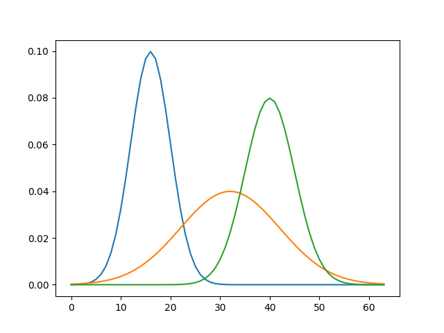
# create a bunch of Gaussian measures on this 1d grid
listMean=[16.,32.,40.]
listStdDev=[4.,10.,5.]
muList=[np.exp(-0.5*((pos-mean)/stddev)**2).ravel() for mean,stddev in zip(listMean,listStdDev)]
# normalize
muList=[mu/np.sum(mu) for mu in muList]


# weights for barycenter computation
weightList=np.array([1.,1.,1.])
weightList=weightList/np.sum(weightList)
nMarginals=weightList.shape[0]

# Simple visualization
for mu in muList:
    plt.plot(mu)
plt.show()

# generate uniform background measure, representing domain on which barycenter is searched
muCenter=np.ones(pos.shape[0])
muCenter=muCenter/np.sum(muCenter)

Now we generate the TMultiScaleSetup objects (one for each marginal measure and one for the center)

# determines how many layers the multiscale representation will have
hierarchyDepth=6

# generate multi scale objects, do not allocate dual variable memory
MultiScaleSetupList=[MultiScaleOT.TMultiScaleSetupGrid(mu,hierarchyDepth,setupDuals=False) for mu in muList]
MultiScaleSetupCenter=MultiScaleOT.TMultiScaleSetupGrid(muCenter,hierarchyDepth,setupDuals=False)

nLayers=MultiScaleSetupCenter.getNLayers()

# list of cost function objects
CostFunctionList=[MultiScaleOT.THierarchicalCostFunctionProvider_SquaredEuclidean(multiX,MultiScaleSetupCenter)\
        for multiX in MultiScaleSetupList]

Now we set up the barycenter container object: it is mostly useful for managing memory of dual variables

BarycenterContainer=MultiScaleOT.TMultiScaleSetupBarycenterContainer(nMarginals)

# assign multi scale objects to barycenter object
for i in range(nMarginals):
    BarycenterContainer.setMarginal(i,MultiScaleSetupList[i],weightList[i])

BarycenterContainer.setCenterMarginal(MultiScaleSetupCenter)


# now allocate dual variables for barycenter problem. the memory is managed by the
# TMultiScaleSetupBarycenterContainer object, not by the separate TMultiScaleSetup objects
BarycenterContainer.setupDuals()

# assign cost function objects to barycenter object
for i in range(nMarginals):
    BarycenterContainer.setCostFunctionProvider(i,CostFunctionList[i])

A few other parameters

errorGoal=1E-3
cfg=MultiScaleOT.TSinkhornSolverParameters()

epsScalingHandler=MultiScaleOT.TEpsScalingHandler()
epsScalingHandler.setupGeometricMultiLayerB(nLayers,1.,4.,2,2)

0

If interested, turn this on

#MultiScaleOT.setVerboseMode(True)

Create and initialize solver object, then solve

SinkhornSolver=MultiScaleOT.TSinkhornSolverBarycenter(epsScalingHandler,0,hierarchyDepth,errorGoal,\
        BarycenterContainer,cfg)
SinkhornSolver.initialize()
SinkhornSolver.solve()

0

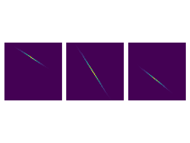
Extract and visualize all couplings

# extract all couplings
couplingData=[SinkhornSolver.getKernelCSRDataTuple(i) for i in range(nMarginals)]
couplings=[scipy.sparse.csr_matrix(cData,shape=(res,res)) for cData in couplingData]

# plot all couplings
fig=plt.figure()
for i in range(nMarginals):
    fig.add_subplot(1,nMarginals,i+1)
    plt.imshow(couplings[i].toarray())
    plt.axis('off')
plt.tight_layout()
plt.show()

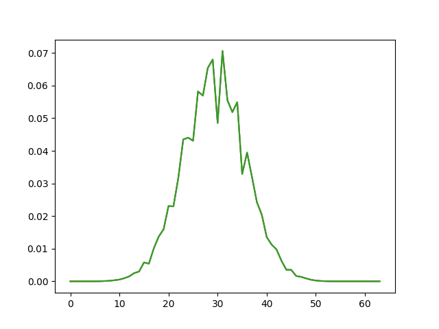
Extract all 2nd marginals (the ones corresponding to the barycenter)

innerMargs=[SinkhornSolver.getMarginalY(i) for i in range(nMarginals)]

# visualize inner marginals (they should all be similar and close to the true barycenter upon successful solving)
# NOTE: the final entropic regularization chosen here is 0.25 (see below)
# which is substantially below the squared distance between two neighbouring pixels (which is 1)
# therefore, the effect of regularization is already pretty weak, and we see discretization artifacts
# which are particularly prominent in the barycenter problem
# see [Cuturi, Peyre: A Smoothed Dual Approach for Variational Wasserstein Problems, DOI: 10.1137/15M1032600,
# Figure 1 for an illustration.

for i in range(nMarginals):
    plt.plot(innerMargs[i])
plt.show()

# print finest eps value:
epsList=epsScalingHandler.get()
epsList[-1][-1]

0.25