1d Sparse Sinkhorn

This example demonstrates on a simple 1-dimensional example the basic usage of the TMultiScaleSetupGrid class for representing a point cloud with a measure on multiple resolution levels and how to use the SparseSinkhorn solver.

import matplotlib.pyplot as plt
import numpy as np
import scipy.sparse
import MultiScaleOT

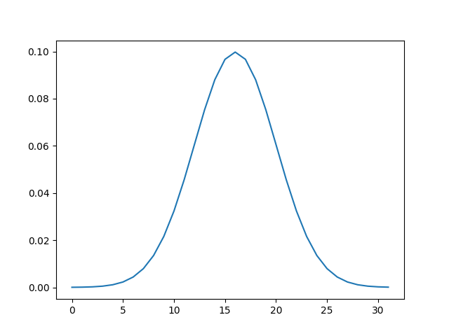
# Generate a 1D Gaussian measure over a 1D list of points
pos=np.arange(32,dtype=np.double).reshape((-1,1))
mu=np.exp(-0.5*((pos-16.)/4.)**2).ravel()
mu=mu/np.sum(mu)


# Simple visualization
plt.plot(mu)
plt.show()

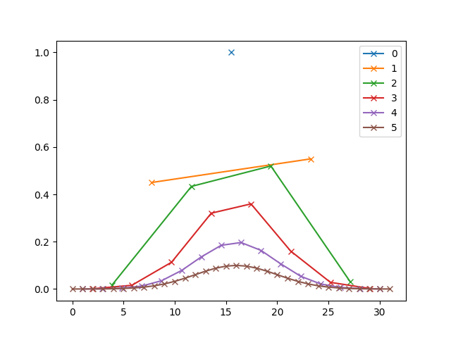
Now we generate the TMultiScaleSetup object

# determines how many layers the multiscale representation will have
hierarchyDepth=5

# generate object
MultiScaleSetup=MultiScaleOT.TMultiScaleSetupGrid(mu,hierarchyDepth)

How many layers are there?

nLayers=MultiScaleSetup.getNLayers()
print(nLayers)

6

How many points are on each layer?

print([MultiScaleSetup.getNPoints(l) for l in range(nLayers)])

[1, 2, 4, 8, 16, 32]

Plot all versions of the measure at all layers. At the coarsest layer it is only a single point with mass 1. At each subsequent finer layer, the mass is split over more points.

for l in range(nLayers):
    posL=MultiScaleSetup.getPoints(l)
    muL=MultiScaleSetup.getMeasure(l)
    plt.plot(posL,muL,marker="x",label=l)
plt.legend()
plt.show()

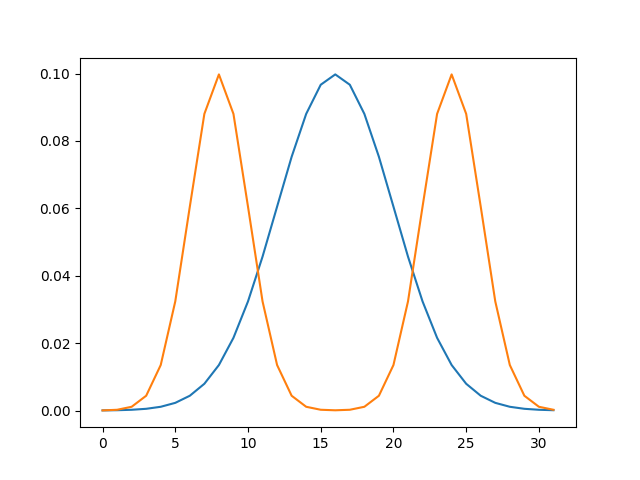
Create a second measure, a sum of two gaussians. Create a corresponding multiscale object. Plot both measures for comparison.

nu=np.exp(-0.5*((pos-8.)/2.)**2).ravel()+np.exp(-0.5*((pos-24.)/2.)**2).ravel()
nu=nu/np.sum(nu)

MultiScaleSetup2=MultiScaleOT.TMultiScaleSetupGrid(nu,hierarchyDepth)

plt.plot(mu)
plt.plot(nu)
plt.show()

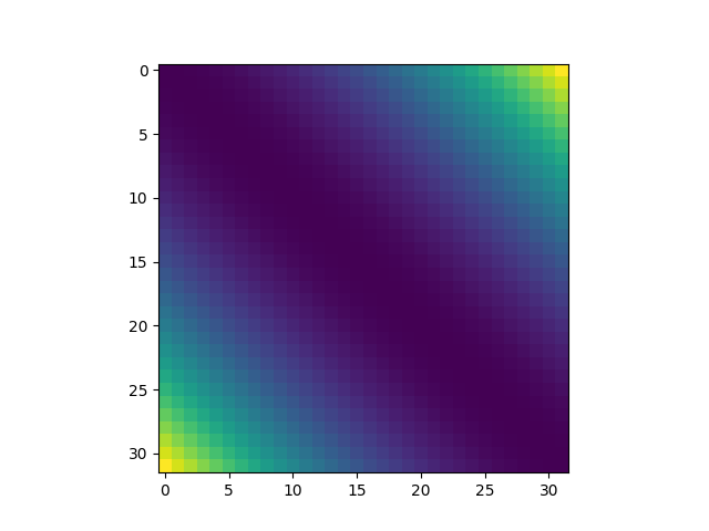
Create a cost function object for the two measures. Evaluate all pairwise costs and display as image.

costFunction=MultiScaleOT.THierarchicalCostFunctionProvider_SquaredEuclidean(
        MultiScaleSetup,MultiScaleSetup2)

# number of points in the two measures:
xres=mu.shape[0]
yres=nu.shape[0]

c=np.array([[costFunction.getCost(hierarchyDepth,x,y) for y in range(yres)] for x in range(xres)])

plt.imshow(c)
plt.show()

Create an epsilon scaling object. Choosing the proper values for epsilon scaling and the scheduling over the multiple layers is not trivial. The following parameters should work well on most Wasserstein-2-type problems.

epsScalingHandler=MultiScaleOT.TEpsScalingHandler()
epsScalingHandler.setupGeometricMultiLayerB(nLayers,1.,4.,2,2)

# Check which values for epsilon scaling have been generated. This returns a list of eps values to be used on each layer.
print(epsScalingHandler.get())

[array([4096., 2048., 1024.]), array([1024.,  512.,  256.]), array([256., 128.,  64.]), array([64., 32., 16.]), array([16.,  8.,  4.]), array([4.  , 2.  , 1.  , 0.5 , 0.25])]

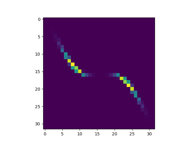
Now generate Sinkhorn solver object, initialize, solve, extract optimal coupling and convert it to scipy.sparse.csr_matrix. Visualize optimal coupling as image.

# error goal
errorGoal=1E-3
# Sinkhorn solver object
SinkhornSolver=MultiScaleOT.TSinkhornSolverStandard(epsScalingHandler,
        0,hierarchyDepth,errorGoal,
        MultiScaleSetup,MultiScaleSetup2,costFunction
        )

# initialize and solve
SinkhornSolver.initialize()
SinkhornSolver.solve()

# extract optimal coupling
kernelData=SinkhornSolver.getKernelCSRDataTuple()
kernel=scipy.sparse.csr_matrix(kernelData,shape=(xres,yres))

plt.imshow(kernel.toarray())
plt.show()

Print the optimal transport cost part of the primal objective (cost function integrated against optimal coupling) and compare it with manually computed value.

print(SinkhornSolver.getScoreTransportCost())
print(np.sum(kernel.toarray()*c))

23.965531931307662
23.96553193130768