2d Image Interpolation: Hellinger–Kantorovich distance

This example computes the Hellinger–Kantorovich unbalanced optimal transport between two simple 2-dimensional images and then generates a simple approximation of the displacement interpolation

import time
import matplotlib.pyplot as plt
import numpy as np
import scipy.sparse
import MultiScaleOT

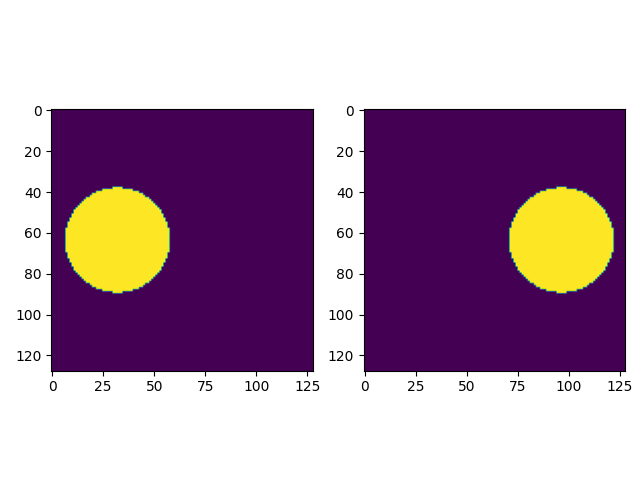
# Create two images: two disks with equal areas

def createImage(size,posX,posY,radX,radY,intensity):
    posXImg=np.zeros((size,size),dtype=np.double)
    posXImg[...]=np.arange(size).reshape((-1,1))-posX
    posYImg=np.zeros((size,size),dtype=np.double)
    posYImg[...]=np.arange(size).reshape((1,-1))-posY

    result=(posXImg**2/radX**2+posYImg**2/radY**2)<=1.
    result=result.astype(np.double)
    result*=intensity
    return result

hierarchyDepth=7 # feel free to play with this value, up to 7 (i.e. 128x128 images) it should be quite low-weight
n=2**hierarchyDepth
nLayers=hierarchyDepth+1
# create two images: a disk on the left, and one on the right, with equal areas

# img1
img1=createImage(n,n/2-0.5,0.25*n,0.2*n,0.2*n,1.)
img1=img1/np.sum(img1)

# img2
img2=createImage(n,n/2-0.5,0.75*n,0.2*n,0.2*n,1.)
img2=img2/np.sum(img2)

fig=plt.figure()
fig.add_subplot(1,2,1)
plt.imshow(img1)
fig.add_subplot(1,2,2)
plt.imshow(img2)
plt.tight_layout()
plt.show()

Aux function for extracting weighted point clouds from images

def extractMeasureFromImage(img,zeroThresh=1E-14):
    dim=img.shape

    pos=np.zeros(dim+(2,),dtype=np.double)
    pos[:,:,0]=np.arange(dim[0]).reshape((-1,1))
    pos[:,:,1]=np.arange(dim[1]).reshape((1,-1))
    pos=pos.reshape((-1,2))
    keep=(img.ravel()>zeroThresh)
    mu=img.ravel()[keep]
    pos=pos[keep]
    return (mu,pos)

# extract measures from images
mu1,pos1=extractMeasureFromImage(img1)
mu2,pos2=extractMeasureFromImage(img2)

Setup multi-scale solver

# set a scale value for the Hellinger--Kantorovich transport
kappa=n*0.75

# generate multi-scale representations
MultiScaleSetup1=MultiScaleOT.TMultiScaleSetup(pos1,mu1,hierarchyDepth,childMode=0)
MultiScaleSetup2=MultiScaleOT.TMultiScaleSetup(pos2,mu2,hierarchyDepth,childMode=0)
# generate a cost function object
costFunction=MultiScaleOT.THierarchicalCostFunctionProvider_SquaredEuclidean(
        MultiScaleSetup1,MultiScaleSetup2,HKmode=True,HKscale=kappa)
# eps scaling
epsScalingHandler=MultiScaleOT.TEpsScalingHandler()
epsScalingHandler.setupGeometricMultiLayerB(nLayers,1.,4.,2,2)

# error goal
errorGoal=1E-1
# sinkhorn solver object
SinkhornSolver=MultiScaleOT.TSinkhornSolverKLMarginals(epsScalingHandler,
        0,hierarchyDepth,errorGoal,
        MultiScaleSetup1,MultiScaleSetup2,costFunction,kappa**2
        )

Solve

t1=time.time()
SinkhornSolver.initialize()
print(SinkhornSolver.solve())
t2=time.time()
print("solving time: ",t2-t1)

0
solving time:  10.413557052612305

compare with full primal score: (this should be large wrt errorGoal)

SinkhornSolver.getScorePrimalUnreg()

3661.894102392003

Extract coupling data in a suitable sparse data structure

couplingData=SinkhornSolver.getKernelPosData()
res1=mu1.shape[0]
res2=mu2.shape[0]

# need to compute marginals of transport plan (are different from mu1,mu2 in unbalanced transport)
couplingDataPos=couplingData.getDataTuple()
couplingMatrix=scipy.sparse.coo_matrix((couplingDataPos[0],(couplingDataPos[1],couplingDataPos[2])),shape=(res1,res2))
nu1=np.array(couplingMatrix.sum(axis=1)).ravel()
nu2=np.array(couplingMatrix.sum(axis=0)).ravel()

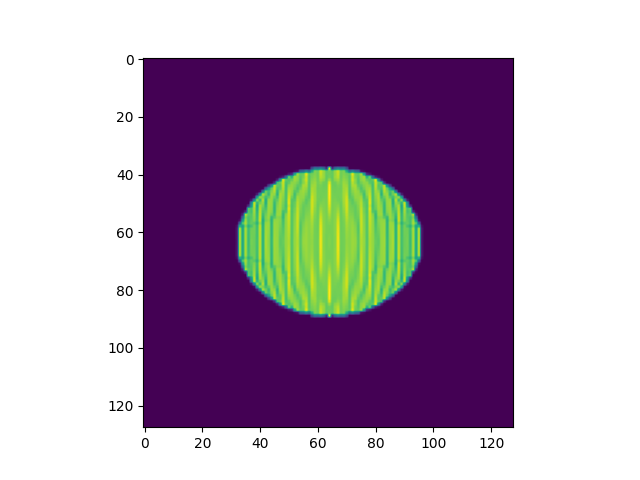
# we plug this into a simple routine for approximating the displacement interpolation at some time t
t=0.5
interpData=MultiScaleOT.interpolateEuclideanHK(couplingData,nu1,nu2,mu1,mu2,pos1,pos2,t,kappa)
# interpData is a container of particle masses and coordinates
# these can be extracted via interpData.getDataTuple()
muT,posT=interpData.getDataTuple()

rasterize to image

reImg=np.zeros((n,n),dtype=np.double)
# rasterize
MultiScaleOT.projectInterpolation(interpData,reImg)
# show rasterization
plt.imshow(reImg)
plt.show()

now do this for a whole sequence of times

nT=10
tList=np.linspace(0.,1.,num=nT)
fig=plt.figure(figsize=(nT*2,2))
for i,t in enumerate(tList):
    fig.add_subplot(1,nT,i+1)

    # create displacement interpolations and rasterize them to image
    interpData=MultiScaleOT.interpolateEuclideanHK(couplingData,nu1,nu2,mu1,mu2,pos1,pos2,t,kappa)

    reImg=np.zeros((n,n),dtype=np.double)
    MultiScaleOT.projectInterpolation(interpData,reImg)

    plt.imshow(reImg)
    plt.axis("off")
plt.tight_layout()
plt.show()

now re-run this for different values of kappa

for kappaPre in [0.625,0.5,0.375,0.25]:
    kappa=kappaPre*n


    costFunction.setHKscale(kappa)
    SinkhornSolver.setKappa(kappa**2)
    SinkhornSolver.solve()

    couplingData=SinkhornSolver.getKernelPosData()
    couplingDataPos=couplingData.getDataTuple()
    couplingMatrix=scipy.sparse.coo_matrix((couplingDataPos[0],(couplingDataPos[1],couplingDataPos[2])),shape=(res1,res2))
    nu1=np.array(couplingMatrix.sum(axis=1)).ravel()
    nu2=np.array(couplingMatrix.sum(axis=0)).ravel()

    nT=10
    tList=np.linspace(0.,1.,num=nT)
    fig=plt.figure(figsize=(nT*2,2))
    for i,t in enumerate(tList):
        fig.add_subplot(1,nT,i+1)

        # create displacement interpolations and rasterize them to image
        interpData=MultiScaleOT.interpolateEuclideanHK(couplingData,nu1,nu2,mu1,mu2,pos1,pos2,t,kappa)

        reImg=np.zeros((n,n),dtype=np.double)
        MultiScaleOT.projectInterpolation(interpData,reImg)

        plt.imshow(reImg)
        plt.axis("off")
    plt.tight_layout()
    plt.show()

• 
• 
• 
•